2.1 Change in Arithmetic and Geometric Sequences

2.1.A

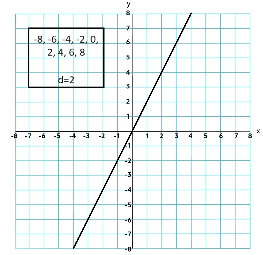
Sequence: a function from the whole numbers to the real numbers. Consequently, the graph of a sequence consists of discrete points instead of a curve

Arithmetic: a function with a common difference, or constant rate of change. General Form: d = common diference and a_k is the kth term in the sequence

a_n = a₀ + dn

a_n = a_k + d(n - k)

2.1.B

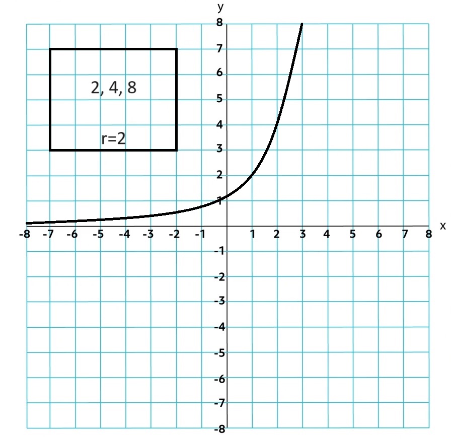
Geometric: a function with a common ratio or constant proportional change. General Form: d = common diference and g_k is the kth term in the sequence

g_n = g₀rⁿ

g_n = g_kr^{(n - k)}

2.2 Change in Linear and 3 Exponential Functions

2.2.A

Linear: form f(x) = b + mx is similiar to the arithmetic sequence in form a_n = a_k + dn. b or a_n are the initial values, added with the constant rate of change, slope (m or d)

Another form can be Arithmetic a_n = a_k+ d(n - k) base off the known difference d and the kth term and linear form f(x) = y_i+ m(x - x_i) base off the known slope m and point (x_i, y_i).

Exponential: form f(x) = ab^x is similiar to the geometric sequence in form g_n = g₀rⁿ. a or g₀ are the initial values, times the repeated constant proportion (b or r)

Another form can be Geometric g_n = g_kr^{(n - k)} based off the known ratio r and a kth term and exponential form f(x) = y_ir^{(x - x_i)} based off the known ratio r, and point (x_i, y_i)

2.2.B

Geometric Sequence: has common raio r denoted by g_n and is given by g_n = g₀rⁿ where g₀ is the initial value or g_n = g_kr^{(n - k)} where k is the kth value.

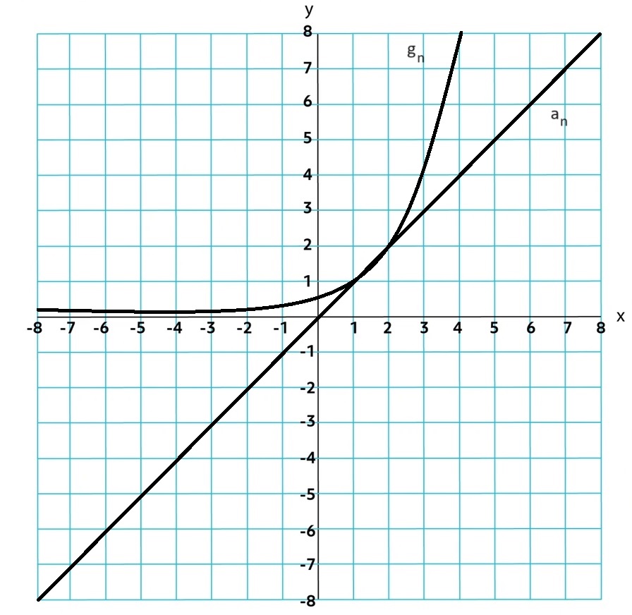
Increasing arithmetic sequences increase equally with each step, whereas increasing geometric sequences increase by a larger amount with each successive step.

2.3 Exponential Functions

2.3.A

Exponential Form: f(x) = ab^x; When a > 0 and b > 1, the exponential function is said to demonstrate exponential growth. When a > 0 and 0 < b < 1, the exponential function is said to demonstrate exponential decay.

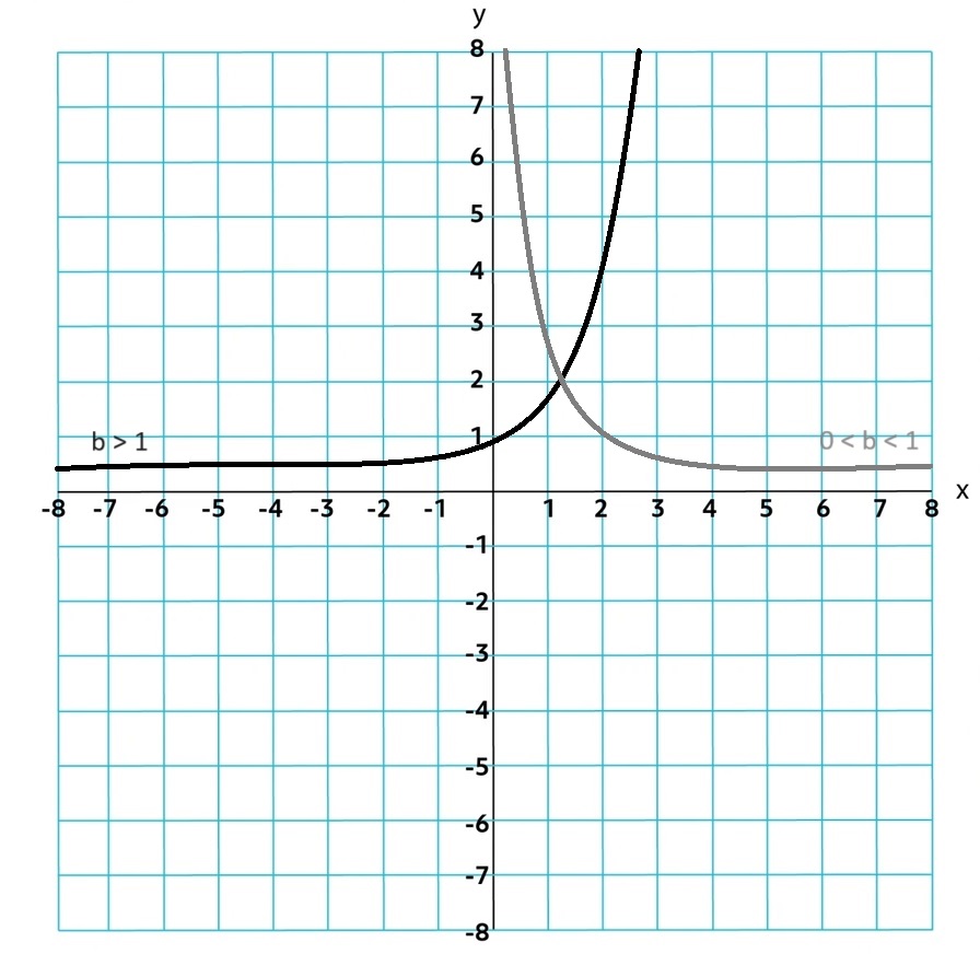
An exponential function with natural nummbers as input values means the domain is all real numbers. They are always concave up or down and always increasing or decreasing. Over Closed intervals there are extrema but not POI.

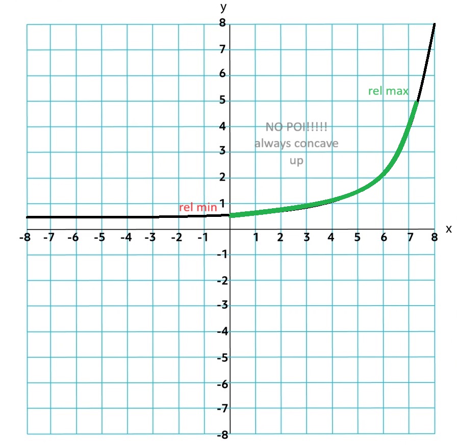
Exponential functions need to be proportional over equal-length input-value intervals even if g(x) is shifted up k units. g(x) = f(x) + k

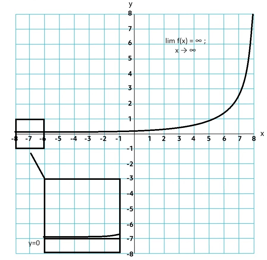
Limit Notation: As the input values increase or decrease without bound, the output values will increase or decrease without bound or will get arbitrarily(extremly close) close to zero. That is, for an exponential function in general form, lim ab^x = ∞; x → ±∞, lim ab^x = −∞; x → ±∞, lim ab^x = 0; x → ±∞.

2.4 Exponential Function Manipulation

2.4.A

The product property for exponents states that b^mbⁿ = b ^{(m + n)}. Graphically, this property implies that every horizontal translation of an exponential function, f(x) = b^{(x + k)}, is equivalent to a vertical dilation, f(x) = b^{(x + k)} = b^xb^k = ab^x, where a = b^k .

The power property for exponents states that (b^m)ⁿ = b^(mn) . Graphically, this property implies that every horizontal dilation of an exponential function, f(x) = b^(cx) , is equivalent to a change of the base of an exponential function, f(x) = (b^c)^x , where bc is a constant and c ≠ 0.

The negative exponent property states b^-n = ¹⁄_bⁿ

The value of an exponential expression involving an exponential unit fraction, such as b^(1/k) where k is a natural number, is the kth root of b, when it exists.

2.5 Exponential Function Context and Data Modeling

2.5.A

Exponential Function: models repeated multiplication of a constant to an initial value over equal length input-values.

An exponential function model can be constructed from an appropriate ratio and initial value or from two input-output pairs. The initial value and the base can be found by solving a system of equations resulting from the two input-output pairs.

f(x) = ab^x

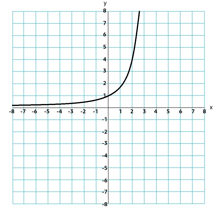
Can be graphed using the exponential regression function on your calculator

You can use exp reg in your calculator

1. stat → edit

2. fill out the L₁(x) and L₂(y)

3. stat → calc → exp reg

4. go to y= and y₁

5. vars → Statistics → EQ → RegEQ

Natural base: e, ~2.718, is often used to model contextual senarios as a base. e^x

2.5.B

base b: growth factor, unit of change in the input values related to the percentage of change in the context.

Ex.

If d represents number of days and the base of f(d) = 2^d then the quantity increases by a actor of 2 every day. Equivalent form f(d) = (2⁷)^(d/7) indicates the quantity by a factor of 2⁷ every week

Exponential models can be used to predict values for the dependent variable, depending on the contextual constraints on the domain.

2.6 Competing Function 3 Model Validation

2.6.A

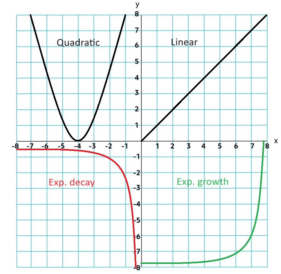
Two variables in a data set that demonstrate a slightly changing rate of change can be modeled by linear, quadratic, and exponential function models. !!Use context clues to determine which graph is more applicable!!

2.6.B

A model is justified as appropriate for a data set if the graph of the residuals of a regression, the residual plot, appear without pattern.

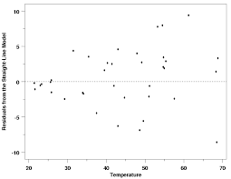
The difference between the predicted and actual values is the error in the model. Depending on the data set and context, it may be more appropriate to have an underestimate or overestimate for any given interval.

2.7 Composition of Functions

2.7.A

If f and g are functions, the composite function f ◦ g maps a set of input values to a set of output value. The output values of g are used as input values for f. For this reason, the domain of the composite function is restricted to those input values of g for which the corresponding output value is in the domain of f. (f ◦ g)(x) can also be represented as f(g(x)). You can calculate or estimate graphically, nucerically, analytically, or verbally using g's ouput values as f's input values

f ◦ g & g ◦ f are typically different funcitions. However, if f(x) = x then g(f(x)) = f(g(x)) = g(x).

!!This is because f(x) = x is the identity function!!

2.7.B

Function composition is useful for relating two quantities that are not directly related by an existing formula. You can contruct by sustituting all values of x in f for g(x).

f(g(x)) or f ◦ g is constucted by (x, f(g(x))).

ex. f(x) = x + 2; g(x) = 3x

f(g(5))

f(g(x)) = 3x + 2

f(g(5)) = 3 x 5 + 2

=17

2.7.C

When properly decomposed, the variable in one function should replace each instance of the function with which it was composed.

An additive transformation of a function, f , that results in vertical and horizontal translations can be understood as the composition of g (x) = x + k with f .

A multiplicative transformation of a function, f , that results in vertical and horizontal dilations can be understood as the composition of g (x) = kx with f .

2.8 Inverse Functions

2.8.A

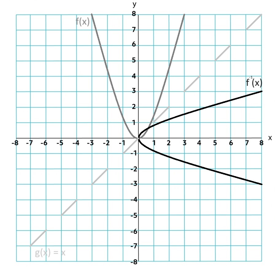
If a function is one-to-one, each ouput has a specific input, it has an inverse function or a function that is invertible.

Inverse Function: f^-1, maps out ouput values of the function f on its invertible domain to their corresponding input values. f(a) = b, then f^-1(b) = a. Input to Output pairs f = (a, b) f^-1 = (b, a)

2.8.B

Identity function: f(f^-1(x)) = f^-1(f(x)) = x

The range of f is the domain of f^-1 and the domain of f is the range of f^-1. Reversed input-output pairs; that is, (a, b) corresponds to (b, a). Reverse the roles of the x and y-axes for y = f^-1(x) from y = f(x) by reflecting it over the graph h(x) = x.

In order to find the inverse, swap the x and y in the equation.

If f(x) = x³ + 8, find f^-1(x)

f(x) = x³ + 8

x = y³ + 8

x - 8 = y³

³√(x - 8) = ³√y³

³√(x - 8) = y

f^-1(x) = ³√(x - 8)

Watch out!! Contextual restrictions may also apply to the inverse.

2.9 Logarithmic Expressions

2.9.A

log_bc = a, where base b must be exponentially raised by a in rder to obtain c; b^a = c only when a and c are constants, b > 0, and b ≠ 1.

logc = log₁₀c = common log

lnc = log_ec = natural log

Values can be calculated or estimated through the use of technology or YOUR BRAIN!!

Logarithmic scale has a multiplicative change, the units could be: 10⁰, 10¹, 10²...

2.10 Inverses of Exponential Functions

2.10.A

General form of Log functions are f(x) = alog_bx, where b > 0, b ≠ 1, a ≠ 0.

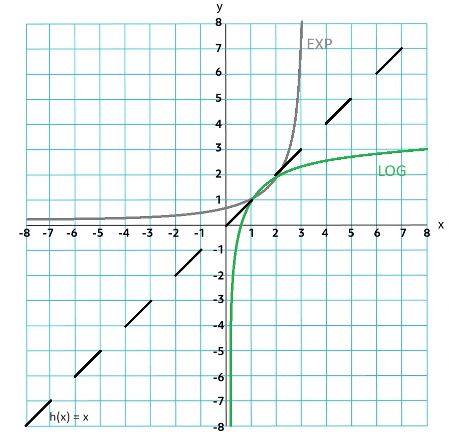
Exponential and Logarithmic functions have an inverse relationship with their inputs and outputs. Exponential growth is characterized by output values changing multiplicatively as input values change additively, whereas logarithmic growth is characterized by output values changing additively as input values change multiplicatively.

The graph of the logarithmic function f(x) = log_bx, where b > 0 and b ≠ 1, is a reflection of the graph of the exponential function g(x) = b^x, where b > 0 and b ≠ 1, over the graph of the identity function h(x) = x. (s, t) for g(x) is (t, s) for f(x).

2.11 Logarithmic Functions

2.11.A

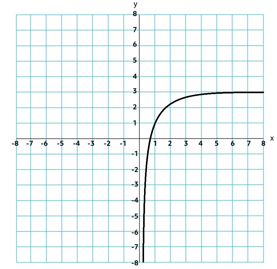
The domain of a log function in general form is any real number greater than zero, and the range is all real numbers.

Because logarithmic functions are inverses of exponential functions, logarithmic functions are also always increasing or always decreasing, and their graphs are either always concave up or always concave down. Consequently, logarithmic functions do not have extrema except on a closed interval, and their graphs do not have points of inflection.

The additive transformation function g (x) = f (x + k), where k ≠ 0, of a logarithmic function f in general form does not have input values that are proportional over equal length output-value intervals. However, if the input values of the additive transformation function, g (x) = f (x + k), of any function f are proportional over equal-length output value intervals, then f is logarithmic.

With their limited domain, logarithmic functions in general form are vertically asymptotic to x = 0, with an end behavior that is unbounded. That is, for a logarithmic function in general form, lim alog_bx = ±∞; x→0⁺, and lim alog_bx = ±∞; x→∞

2.12 Logarithmic Function Manipulation

2.12.A

The product property for logarithms states that log_b(xy) = log_bx + log_by. Graphically, this property implies that every horizontal dilation of a logarithmic function, f(x) = log_b(kx), is equivalent to a vertical translation, f(x) = log_b(kx) = log_bk + log_bx = a + log_bx, where a = log_bk.

The power property for logarithms states that log_bxⁿ = nlog_bx. Graphically, this property implies that raising the input of a logarithmic function to a power, f(x) = log_bx^k , results in a vertical dilation, f(x) = log_bx^k = klog_bx.

The change of base property for logarithms states that log_bx = ^log_ax⁄_logab, where a > 0 and a ≠ 1. This implies that all logarithmic functions are vertical dilations of each other.

Function f(x) = lnx is a logarithmic function with the natural base e; lnx = log_ex

2.13 Exponential and Logarithmic Equations and Inequalities

2.13.A

Properties of exponents, properties of logarithms, and the inverse relationship between exponential and logarithmic functions can be used to solve equations and inequalities involving exponents and logarithms. Check for extraneous solutions by mathematical or contextual limitations

Logarithms can be used to rewrite expressions involving exponential functions in different ways that may reveal helpful information. Specifically, b^x = c^(log_cb)(x)

2.13.B

The function f(x) = ab^{(x - h)}+ k is a combination of additive transformations from the exponential general form f(x) = b^x.

The function f(x) = alog_b(x - h) + k is a combination of additive transformations from the logarithmic general form f(x) = log_bx.

The inverse of y = f(x) can be found by determining the inverse operations to reverse the mapping

2.14 Logarithmic Function Context and Data Modeling

2.14.A

Logarithmic and Exponential functions are inverses so ca be used to model situations involving proportional group or repeated ultiplication over equal length ouptut values.

Logaritmic function model: one real zero or from 2 input-output pairs. Add transformations to f(x) = alog_bx based off characteristics of a context or data set.

You can use log reg in your calculator

1. stat → edit

2. fill out the L₁(x) and L₂(y)

3. stat → calc → log reg

4. go to y= and y₁

5. vars → Statistics → EQ → RegEQ

The natural logarithm function is often useful in modeling real-world phenomena.

Logarithmic function models can be used to predict values for the dependent variable.

2.15 Semi-log Plots

2.15.A

Semi-log plot: one axis is logarithmically scaled. When the y-axis is logarithmically scaled, then the exponentical function will look linear. An advantage of a semi-log plot is that the constant never needs to be added to the dependent variable to reveal an exponential model.

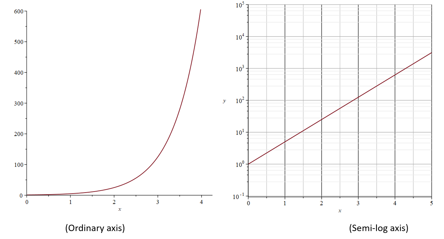
2.15.B

Tequniques to model linear functions can be applied to semi-log graphs.

For an exponential model of the form y = ab^x, the corresponding linear model for the semilog plot is y = (log_nb)x + log_na, where n > 0 n and n ≠ 1. Specifically, the linear rate of change is log_nb, and the initial linear value is log_na.